What Does Orthogonality Mean in PL Design?

Summary

Orthogonality is a pervasive, but tacit, design principle in the PL community. Orthogonal design concepts are ones that don't intersect. A consequence of this is that we can intersect non-orthogonal concepts to find orthogonal pieces. The intersection approach works well when the orthogonal concepts are at an abstraction level lower than the one you're currently at, since it breaks things into smaller pieces.

Orthogonal concepts are useful, because they are maximally independent from each other. Since orthogonal concepts are more distinct from one another, they might be easier to remember and it might be easier to pick the right concept for the job. But we don't have research on that yet.

Orthogonality is a design principle in programming languages (PL) that is part of the tacit knowledge of the research community. Probably every PL researcher knows what orthogonality is when they see it. But you’d be hard-pressed to find a good description of the concept to anyone outside the community. As a result, it’s hard to explain (let alone justify) orthogonality to language, library, and API designers outside of the PL community. In this post I’ll do my best to explain what orthogonality is and why it matters.

First I want to define the scope I’m going to consider. When I was coming up with examples and looking around for other explanations, I found a few different-but-related uses of orthogonality. One use of orthogonality is to describe inputs to a system. Here’s an example of that from The Pragmatic Programmer by Andrew Hunt and David Thomas:

You’re on a helicopter tour of the Grand Canyon when the pilot, who made the obvious mistake of eating fish for lunch, suddenly groans and faints. Fortunately, he left you hovering 100 feet above the ground. You rationalize that the collective pitch lever controls overall lift, so lowering it slightly will start a gentle descent to the ground. However, when you try it, you discover that life isn’t that simple. The helicopter’s nose drops, and you start to spiral down to the left. Suddenly you discover that you’re flying a system where every control input has secondary effects. Lower the left-hand lever and you need to add compensating backward movement to the right-hand stick and push the right pedal. But then each of these changes affects all of the other controls again. Suddenly you’re juggling an unbelievably complex system, where every change impacts all the other inputs. Your workload is phenomenal: your hands and feet are constantly moving, trying to balance all the interacting forces.

This is not the kind of orthogonality I want to discuss.

Another notion of orthogonality can be found in The Art of Unix Programming by Eric S. Raymond:

The problems with non-orthogonality arise when side effects complicate a programmer’s or user’s mental model, and beg to be forgotten, with results ranging from inconvenient to dire. Even when you do not forget the side effects, you’re often forced to do extra work to suppress them or work around them.

This is not a definition of orthogonality, but I chose this quote, because it helps us understand how Eric Raymond thinks about the idea. This notion of orthogonality is related to the previous one, but emphasizes hidden dependencies or side effects in some piece of functionality. I’m not really going to be talking about this either. Instead, I’m going to be discussing orthogonal concepts or language features.

Example 1: Natural Semantic Metalanguage

First I’ll give you a flavor for orthogonality using the example from my Natural Semantic Metalanguage post. The Natural Semantic Metalanguage aims to provide a set of a “orthogonal” primitive words (primes) that can be used to define all other words.

First, here are Oxford Languages definitions of two related words:

• Happy: “feeling or showing pleasure or contentment”
• Contented: “happy and at ease”

For the purposes of this post, I want to you pay attention to the fact that these emotion words are very much not orthogonal. “Happy” and “contented” are defined in terms of each other, for example. This makes it hard to nail down the precise differences in usage.

Let’s contrast this with the NSM “explications” of these words:

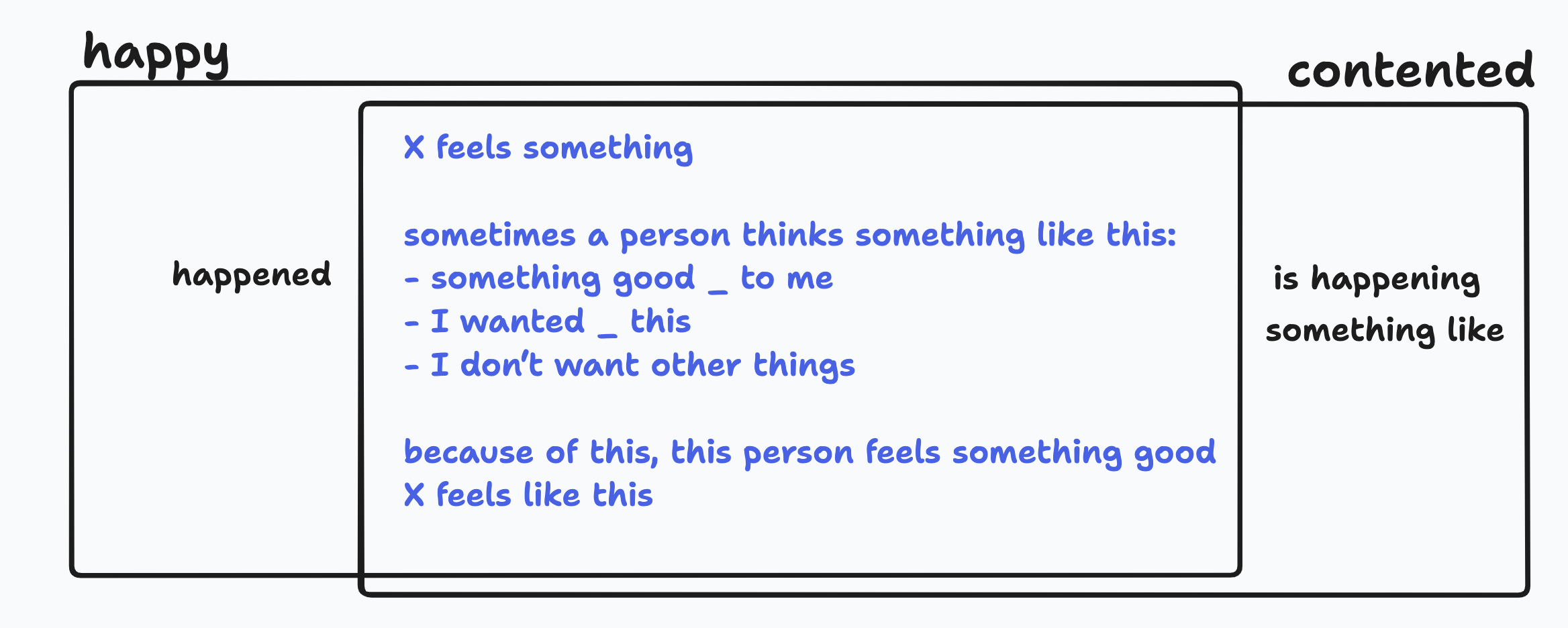
Happy

X feels something

sometimes a person thinks something like this:
- something good happened to me
- I wanted this
- I don’t want other things

because of this, this person feels something good
X feels like this

Contented

X feels something

sometimes a person thinks something like this:
- something good is happening to me
- I wanted something like this
- I don’t want other things

because of this, this person feels something good
X feels like this

Notice that words like “something” and “person” share little or no overlap with other NSM primes. Now we can precisely compare “happy” and “contented”. To get from “happy” to “contented,” we can change “something good happened to me” to “something good is happening to me” and “I wanted this” to “I wanted something like this.”

What are the tradeoffs of the high-level non-orthogonal words “happy” and “contented” and the low-level orthogonal primes? The high-level words are terse, relying on a shared cultural understanding to convey meaning more quickly. On the other hand, high level words may be harder to learn without their lower-level definitions. Moreover, it may be harder to choose the word you really want if you only have high-level descriptions of each emotion. And if you want a new word that captures a different feeling, that’s much harder to do without the low-level language.

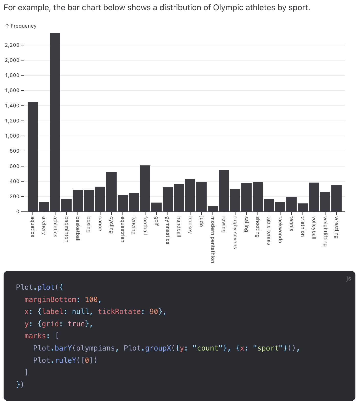
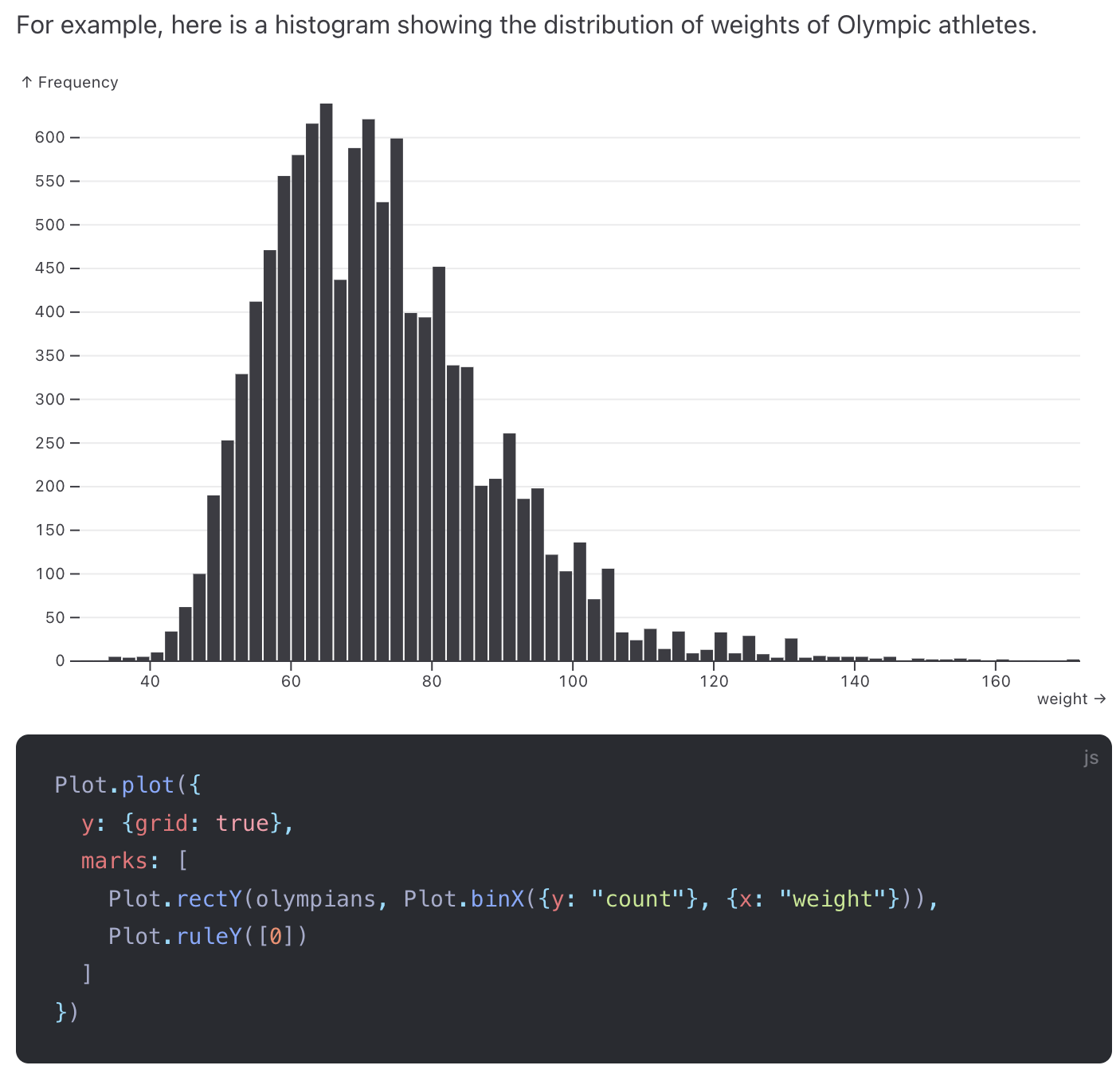
Example 2: Data Visualization Abstractions

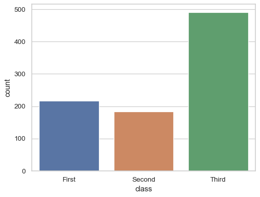
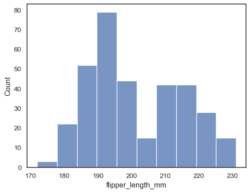
Here’s a similar phenomenon in data visualization abstraction design. Here are two high-level visualization “words” in seaborn, a Python data vis library:

• countplot: “Show the counts of observations in each categorical bin using bars. A count plot can be thought of as a histogram across a categorical, instead of quantitative, variable.”

• histplot: “Plot univariate or bivariate histograms to show distributions of datasets. A histogram is a classic visualization tool that represents the distribution of one or more variables by counting the number of observations that fall within discrete bins.”

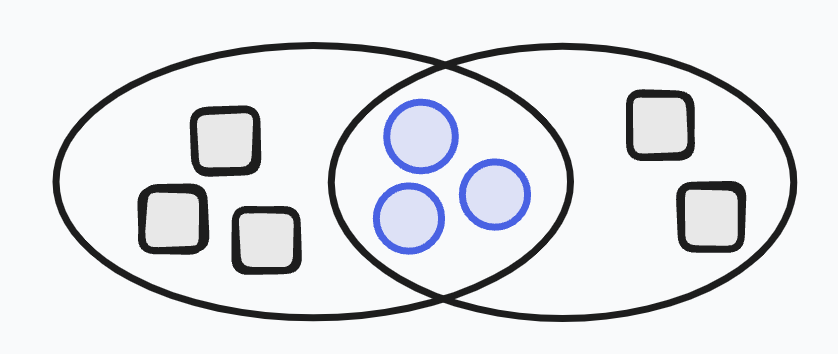
See how these words are similar to the culturally specific emotions above? We even see a count plot defined in terms of a histogram! I want to introduce a way that I think about finding orthogonality in concepts like these: intersection. When two concepts are not orthogonal, their meanings overlap. And when they overlap, we can intersect those two concepts to find some more primitive concepts hiding in their overlap and in their differences. This is a conceptual tool we can use to search for more primitive ideas.

In the case of “happy” and “contented,” it’s challenging to think of their intersection given just their high-level definitions.

But it’s straightforward if we use their NSM explications.

We can play the same game with countplot and histplot. Suppose we don’t yet have a lower-level definition. We can begin to identify similarities and differences. Both use bar marks. Both use some kind of grouping, but the grouping differs between the two. (There are also some default behaviors that we’ll ignore.)

In a grammar of graphics library like Observable Plot, we can express this difference more directly:

We can intersect these definitions to tease apart their similarities and differences.(This can be done systematically for grammars in a process known as “anti-unification.”)

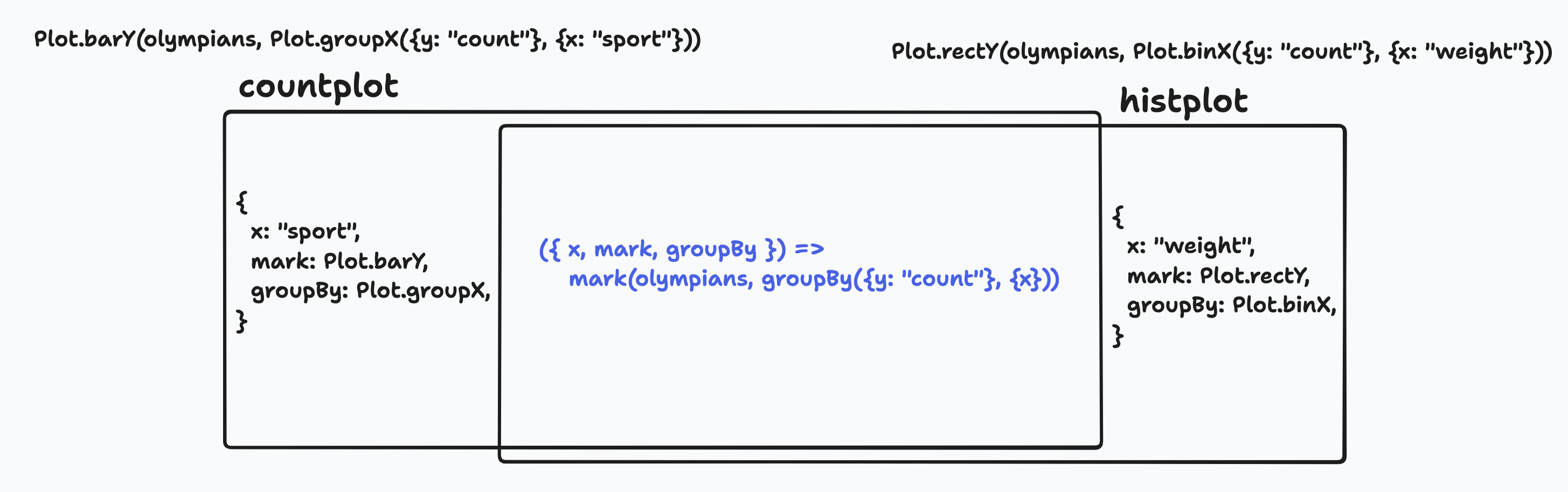
Notice that the field we used changed, the grouping behavior changed, but also the mark changed! This is because in Observable Plot, you use a different mark depending on whether your data is categorical or quantitative.

I want to point out a difference between these two examples. The code example’s intersection and differences can also be written as code. While the NSM explication can be written in English, I didn’t use a standardized format for their intersection or differences. With code we can just use functions applied to different sets of data.

We can take this idea further, though. For example, we could try to intersect groupX and binX. They are both functions that operate on some data and produce grouped data as a result. (Actually this is not true. A transform in Observable Plot is not a function but instead a more complicated object. That’s out of scope for this post.) We could write a higher-order groupBy function and define them kinda like this:

const groupX = (data, field) =>
    groupBy(data, row => row[field])
const binX = (data, field) =>
    groupBy(data, row => Math.floor(row[field] / binWidth) * binWidth)

Bunch of caveats with these definitions as they wouldn’t really work as written, but the point I want to make is that you can keep playing this intersection game, coming across new puzzles to solve and boiling away concepts, leaving the remaining ones more orthogonal.